[인공지능(AI) 기초 다지기] 5. 딥러닝 핵심 기초 (8)

6) Softmax Classification

 

- Discrete Probability Distribution (이산 확률 분포)

• ex) 주사위, 가위바위보 
• PDF(확률밀도함수, 정규분포) 는 함수의 면적이 확률값
  point 자체는 확률이 아님, 알 수 없음
• PMF(확률질량함수, 이산적인 확률 분포) 에서는 어떤 값 = 확률

 

- Softmax

• max 를 soft 하게 뽑는다 = 합쳐서 1이 되는 값으로 나타냄 = 확률값
  [1, 2, 3] -> max : (0, 0, 1)
                -> softmax : (0.0900, 0.2447, 0.6652)

• 가위를 냈을 때 주먹 / 가위 / 보 를 낼 확률
• 소프트맥스 값은 확률값이 됨

 

- Cross Entropy

• 두 개의 확률 분포가 주어졌을 때 확률 분포가 얼마나 비슷한지 나타낼 수 있는 수치

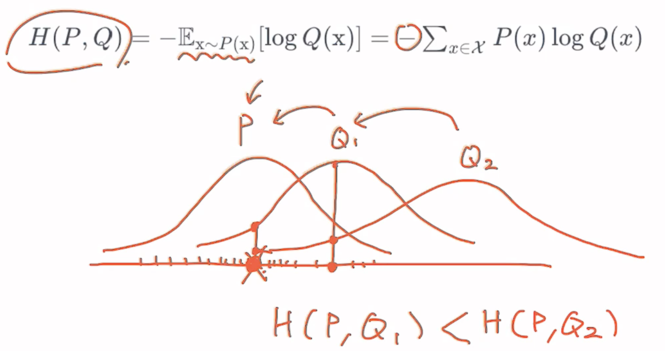
• P : 철수가 가위를 냈을 때 다음에 무엇을 낼지에 대한 확률 분포 함수
• cross entropy 를 최소화 하면 계속해서 Q2 가 Q1, Q1이 P에 가까워짐
  = 모델의 확률 분포 함수는 점점 P 에 근사함

 

- Cross Entropy Loss (Low-level Implementation)

• Pθ(x) <- Q(x)

z = torch.rand(3, 5, requires_grad=True) # uniform random : size = (3, 5)
hypothesis = F.softmax(z, dim=1)
print(hypothesis)
'''
tensor([[0.2645, 0.1639, 0.1855, 0.2585, 0.1277],
        [0.2430, 0.1624, 0.2322, 0.1930, 0.1694],
        [0.2226, 0.1986, 0.2326, 0.1594, 0.1868]], grad_fn=<SoftmaxBackward0>)
'''

• requires_grad=True : gradient 배우게 함
• 2번째 dimension 에 대해서 softmax 수행
  = [0.2430, 0.1624, 0.2322, 0.1930, 0.1694](이미 수행된 결과값) dimension 에 대해서 softmax 수행 
• 결과값은 예측값 (= ^y = prediction)

y = torch.randint(5, (3,)).long()
print(y)
'''
tensor([0, 2, 1]) # one hot vector 의 인덱스 값
'''

• y : 랜덤하게 정답 생성
• class 갯수 : 5
  sample 갯수 : 3
• y는 각각 샘플에 대한 정답의 인덱스임
• 즉, 정답은 hypothesis 의 (0,0), (1, 2), (2, 1) 값 = [0.2645, 0.2322, 0.1986]

y_one_hot = torch.zeros_like(hypothesis)
y_one_hot.scatter_(1, y.unsqueeze(1), 1) # one hot vector 로 나타낸 것
'''
tensor([[1., 0., 0., 0., 0.],
        [0., 0., 1., 0., 0.],
        [0., 1., 0., 0., 0.]])
'''

cost = (y_one_hot * -torch.log(hypothesis)).sum(dim=1).mean()
print(cost)
'''
tensor(1.4689, grad_fn=<MeanBackward0>)
'''

• 이산 확률 분포 -> one hot vector 로 나타내줌
  |y_one_hot| = (3, 5) = y_one hot 사이즈 = hypothesis 사이즈
• scatter_ : inplace 연산 (새로 메모리 할당하지 않고 y_one_hot 값이 교체됨)
  (1, y.unsqueeze(1), 1) : dimension 1 에 대해서 y.unsqueeze(1) 을 가지고 1 을 뿌려라
• |y| = (3, ) -> |y_unsqueeze| = (3, 1)
• 아까 [0, 2, 1] -> [[0], [2], [1]]
• log : cross entropy 수식
• .sum(dim=1) : sum 하면 (3, 1) 사이즈가 됨 -> 두번째 dimension(=dimension 1) 은 사라짐 -> scalar

 

- Cross Entropy Loss with torch.nn.functional (High-level Implementation)

# low level
torch.log(F.softmax(z, dim=1))

# high level
F.log_softmax(z, dim=1)

# low level
(y_one_hot * -torch.log(hypothesis)).sum(dim=1).mean()

# high level
F.nll_loss(F.log_softmax(z, dim=1), y)

F.cross_entropy(z, y)

• nll = Negative Log Likelihood
• -, .sum(dim=1).mean() = nll_loss
• cross_entropy = log_softmax + nll_loss
  -> softmax 를 포함함
• 뉴럴 네트워크에서 확률값을 뱉어줘야 함 -> softmax 이전의 값을 필요할 때가 있음
• 예측하는 과정에서 확률값을 구하기 위해서 다시 softmax 를 취해야 할 수도 있음

 

- Training Example

x_train = [[1, 2, 1, 1],
           [2, 1, 3, 2],
           [3, 1, 3, 4],
           [4, 1, 5, 5],
           [1, 7, 5, 5],
           [1, 2, 5, 6],
           [1, 6, 6, 6],
           [1, 7, 7, 7]]
y_train = [2, 2, 2, 1, 1, 1, 0, 0]
x_train = torch.FloatTensor(x_train)
y_train = torch.LongTensor(y_train)

• |x_train| = (m, 4)
  |y_train| = (m, )
• 4차원의 vector 를 받아서 어떤 class 인지 예측 
• y_train : one hot vector 로 나타냈을 때 1이 있는 인덱스 값 -> discrete 하기 때문에

# Low-level Cross Entropy

# 모델 초기화
W = torch.zeros((4, 3), requires_grad=True)
b = torch.zeros(1, requires_grad=True)

# optimizer 설정
optimizer = optim.SGD([W, b], lr=0.1)

nb_epochs = 1000
for epoch in range(nb_epochs + 1):
    
    # Cost 계산 
    hypothesis = F.softmax(x_train.matmul(W) + b, dim=1) # matmul or .mm or @
    y_one_hot = torch.zeros_like(hypothesis)
    y_one_hot.scatter_(1, y_train.unsqueeze(1), 1)
    cost = (y_one_hot * -torch.log(F.softmax(hypothesis, dim=1))).sum(dim=1).mean()
    
    # Cost 로 H(x) 계산
    optimizer.zero_grad()
    cost.backward() # loss 값 backpropagation
    optimizer.step() # gradient descent
    
    # 100번 마다 log 출력
    if epoch % 100 == 0:
        print("Epoch {:4d}/{} Cost: {:.6f}".format(
            epoch, nb_epochs, cost.item() 
        ))

• # samples = m (number of samples)
  # classes = 3
  dim = 4 (입력 벡터)
• 하나의 linear layer 만 (4에서 3으로 가는 linear layer)
• cost.item() : loss 값 -> 점점 떨어지는 것 확인

# F.cross_entropy

# 모델 초기화
W = torch.zeros((4, 3), requires_grad=True)
b = torch.zeros(1, requires_grad=True)

# optimizer 설정
optimizer = optim.SGD([W, b], lr=0.1)

nb_epochs = 1000
for epoch in range(nb_epochs + 1):
    
    # Cost 계산 
    z = x_train.matmul(W) + b
    cost = F.cross_entropy(z, y_train)
    
    # Cost 로 H(x) 계산
    optimizer.zero_grad()
    cost.backward()
    optimizer.step()
    # 100번 마다 log 출력
    if epoch % 100 == 0:
        print("Epoch {:4d}/{} Cost: {:.6f}".format(
            epoch, nb_epochs, cost.item()
        ))

• one hot vector 만드는 과정 생략
• optimizer.step() : gradient descent 를 통해서 cross entropy 함수(=loss)를 minimize 함
  = 확률 분포 P 에 근사

 

- Higher Implementation with nn.Module

class SoftmaxClassifierModel(nn.Module):
    def __init__(self):
        super().__init__()
        self.linear = nn.Linear(4, 3) # output이 3
        
    def forward(self, x):
        return self.linear(x)

• linear layer : 4개의 input을 받아서 3개의 class에 대한 확률값
• forward (=진행) : linear layer 통과
• |x| = (m, 4) : m = 샘플 숫자
  -> return 값 (linear layer 통과한 후 값) : (m, 3)

# 모델 초기화
W = torch.zeros((4, 3), requires_grad=True)
b = torch.zeros(1, requires_grad=True)

# optimizer 설정
optimizer = optim.SGD(model.parameters(), lr=0.1)

nb_epochs = 1000
for epoch in range(nb_epochs + 1):
    
    # H(x) 계산
    prediction = model(x_train)
    
    # Cost 계산 
    cost = F.cross_entropy(prediction, y_train)
    
    # Cost 로 H(x) 계산
    optimizer.zero_grad()
    cost.backward()
    optimizer.step()
    
    # 100번 마다 log 출력
    if epoch % 100 == 0:
        print("Epoch {:4d}/{} Cost: {:.6f}".format(
            epoch, nb_epochs, cost.item()
        ))

• prediction : model 을 통과시킴
  -> |x_train| = (m, 4)
       |prediction| = (m, 3)
• y_train : index 값 (아직 one hot vector X)
  |y_train| = (m, )
• cost 는 scalar 값
• model.parameters() 에 gradient descent 채워짐

• Logistic Regression 과 매우 유사 (0 / 1  두 가지 class 만 있는 discrete classification)
• Softmax Classification 은 multinomial 확률 분포  
• binary 할 때는 logistic 함수를 쓰고 = BCE(binary cross entropy) loss + sigmoid
• 여러 개 class 가 있다면  = CE + softmax